
This article is the first installment of a three part series in which we will examine oscilloscope measurements such as the ones available in hardware within the ZTEC family of modular oscilloscopes. Many oscilloscope users take advantage of only a small fraction of the powerful features available to them. In addition, selecting the right measurement from a catalog of possibilities and accurately interpreting the results can lead to confusion and mistakes. This series of articles is intended to help users understand oscilloscope measurements more completely in order to avoid common pitfalls.
Digital storage oscilloscopes vary greatly among vendors in terms of form factor (stand-alone, PXI, VXI, PCI, etc), resolution (8-bit, 12-bit, 16-bit, etc), acquisition rates (1 MS/sec, 1 GS/sec, 40 GS/sec, etc), functionality (advanced triggering, deep memory, self-calibration, etc.), and more. One aspect that separates true oscilloscopes from most PC-based, modular digitizers is the ability to make measurements in hardware on an onboard processor. The available measurements also differ from one oscilloscope to another, although this paper will cover a large segment of them. In addition, the algorithms used to complete the measurements may differ slightly among vendors. This paper will focus on the measurements and algorithms used in ZTEC modular oscilloscopes, but most of these concepts are universal.
Oscilloscope measurements can be sorted into the following three categories:
- Vertical-Axis
- Horizontal-Axis
- Frequency-Domain
Part one of the series will focus on vertical-axis measurements
Vertical-axis measurements analyze the vertical component of the applied signal. These measurements most often describe a signal in terms of a voltage level. However, they can also correspond to current, power, or any other physical phenomena converted to voltage via a probe or transducer. Some common vertical-axis measurements include Amplitude, Peak-To-Peak, Average, and RMS measurements.
Vertical Resolution and Accuracy
The resolution and accuracy of an oscilloscope can affect measurements greatly, so it’s important to understand these limitations. An oscilloscope with an 8-bit analog-to-digital converter (ADC) has 28 (256) levels available while a 16-bit ADC has 216 (65536) levels. Thus, a 16-bit oscilloscope has 256 times more resolution than an 8-bit oscilloscope. Since only finite levels are available to represent the signal, there is a quantization error of 1 least significant bit (LSB). To find the minimum detectable voltage change (code width), divide the input range by the number of levels. Figure 1 depicts a 16-bit oscilloscope digitizing an 8 Vpp square wave with a 100 mV ripple voltage. In this case, the oscilloscope’s code width is (10/65536) 150 uV which allows it to produce a good representation of both the large and small signals. An 8-bit oscilloscope’s code width would be only (10/256) 39 mV, so it could not show the 100 mV component adequately. Changing the input range setting to 250 mVpp would improve the performance, reducing the code width to (0.25/256) 1 mV.
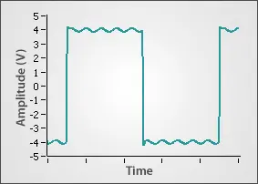
Figure 1: Signal with Large & Small Components
The dynamic range of an oscilloscope refers to how well the instrument can detect small signals in the presence of large signals and is expressed in decibels (dB). It is limited by the quantization error and all other noise sources such as background noise, distortion, spurious signals, etc. The equation for computing the dynamic range is:

Vmax is the maximum voltage that must be acquired and Vres is the minimum resolution that can be seen. A good rule of thumb is that every bit of resolution equals 6 dB of dynamic range. An 8-bit instrument’s theoretical maximum dynamic range is 48 dB, but it is significantly less once all limitations are considered. Accuracy refers to the oscilloscope’s ability to represent the true value of a signal. An oscilloscope with high resolution, does not necessarily translate into giving an accurate result. Accuracy and resolution are related though, because the achievable accuracy of an instrument is limited by the resolution of the ADC.
The factors that reduce the accuracy of an oscilloscope can be mostly lumped into high- and low-frequency errors. Noise is generally the cause of high-frequency errors, while low-frequency errors are caused by drift stemming from temperature, aging, bias currents, etc. High-frequency errors can usually be removed by oversampling and averaging. Low-frequency errors often require the calibration of the instrument, either internally or through a factory calibration.
Relative vs. Absolute Measurements
An oscilloscope’s accuracy is often specified in terms of gain accuracy and offset accuracy. Gain accuracy is related to how well it handles high-frequency noise and can be called its relative accuracy. Offset accuracy is related to how well it handles the low-frequency issues and can be referred to as absolute accuracy. Figure 2 shows a real and measured 1 Vpp sine wave. Notice that the measured Amplitude is 0.99 V which equates to a gain error of 0.01 V or 1%. The measured signal is also offset 0.02 V for a 2% offset error.
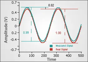
Figure 2: Gain & Offset Errors
Vertical-axis measurements can either be relative or absolute in nature. Relative measurements compare two voltages within the same signal. Amplitude is an example of a relative measurement because it returns the difference between the high and low voltage. The Amplitude of a 1 Vpp sine wave will be the same when it is centered at zero or has an offset of 5 V. Therefore, relative measurements are unaffected by the offset error. Absolute measurements are a representation of their real-world value and are affected by gain and offset errors. The Average measurement is an example of an absolute measurement.
Amplitude vs. Peak-To-Peak
Two vertical-axis measurements that are often confused are Amplitude and Peak-To-Peak. This is understandable because they are identical for all types of signals, except a pulse signal. Figure 3 shows the difference between the Amplitude and Peak-To-Peak (PTPeak) for a pulse signal. Peak-To-Peak returns the difference between the extreme Maximum and Minimum values, while the Amplitude returns the difference between where the pulse settles at the top (High) and bottom (Low) of the signal. The other measurements shown--Rise Overshoot (ROV), Rise Preshoot (RPR), Fall Overshoot (FOV), and Fall Preshoot (FPR)--are only valid when measuring pulses.
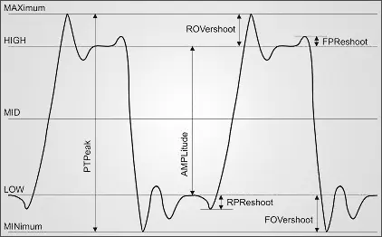
Figure 3: Vertical Axis Measurements [1]
The measurements shown in Figure 3 are computed on the oscilloscope processor using a histogram. Figure 4 shows how the pulse signal in Figure 3 is represented in an 8-bit oscilloscope histogram. The samples are sorted into one of 256 bins, each corresponding to a voltage range. The algorithms simply look for the bit value with the most points for the Low and High measurements and the absolute largest and smallest bit values for the Maximum and Minimum. This allows for an extremely fast computation, but the measurement’s resolution is limited by the quantization error (1 LSB) of the ADC. The accuracy also suffers due to a single sample’s susceptibility to noise.
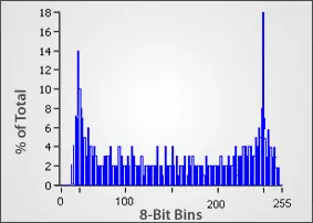
Figure 4: Histogram Processing of a Sine Wave
Root Mean Squared (RMS) & Average
The Direct Current (DC) RMS, Alternating Current (AC) RMS, and Average measurements are methods of characterizing the vertical level and power using the entire waveform.
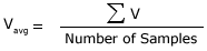
The Average function is the mean vertical level of the entire captured waveform. It can be calculated by taking the sum of all of the voltage levels and dividing that by the number of points as shown:
The DC RMS and AC RMS measurements return the average power of the signal. The DC RMS returns the entire power contained within a signal including AC and DC components. This can also be described as the heating power when applied to a resistor. The AC RMS is used to characterize AC signals by subtracting out the DC power, leaving only the AC power component. The equations for the RMS measurements are as follows:
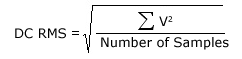
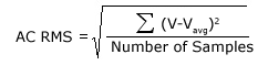
Figure 5 shows these results on a 4 Vpp square wave with 0.5 V of offset.
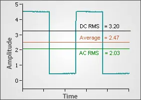
Figure 5: Average & RMS
All three of these measurements are capable of more accuracy than the Amplitude and Peak-To-Peak measurements described in the previous section. The reason for this is that every single point in the waveform is included in the calculation of the Average and RMS measurements. This naturally cancels out noise that may be present in the signal. Additionally, when measuring the Average or RMS values, the more points that are acquired in the waveform, the better the accuracy of the measurements become. The upper bound of the accuracy is determined by the number of bits in the onboard processor. Some oscilloscopes use a 16-bit processor, so these measurements are limited to 16 bits of resolution because the largest number that can be stored on the chip is 16-bits. However, the 64-bit processor on the ZT4611 modular oscilloscope allows users to attain up to 64 bits of resolution. The tradeoff for the higher accuracy is longer computations since more points must be analyzed.
When only a few cycles of a waveform is acquired, it becomes critical to acquire only the full cycles or otherwise the results contain an asymmetric error. Figure 6 shows the same signal as Figure 5 except that an additional (high) half cycle was acquired. The Average and RMS values are offset because of this.
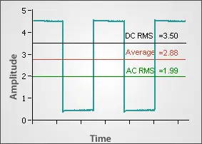
Figure 6: Average & RMS with Partial Cycle
There are a few ways to avoid this circumstance. The best way is to acquire a longer waveform that includes many cycles so that the offset is effectively minimized. This method requires more time and more onboard memory to store the waveform. Another way to solve the problem is to make use of the Cycle RMS or Cycle Average measurements. These calculate the RMS and Average including only the points from the first cycle of the waveform. The third way to solve the problem would be to use a gated measurement. Gated measurements allow the user to choose the points that are included. This can be done by selecting a start and stop time or a start and stop point. Both the Gated By Time and Gated By Points methods require the user to know the period of the waveform to solve the problem shown in Figure 6.
Horizontal-Axis Measuremets
Horizontal-axis measurements involve analyzing the horizontal time axis of the applied signal, and include measurements such as Period, Frequency, and Rise Time. The value returned is usually in time, but can also be expressed as a ratio, radians, or in Hertz.
Horizontal Resolution and Accuracy
The horizontal-axis resolution is limited by the sample rate of the onboard clock. A board with a 1 GS/sec acquisition rate can only achieve a time resolution of 1 / (1 GS/sec) = 1 nsec. Much like the vertical axis, the horizontal-axis accuracy can be reduced by high- and low-frequency errors.
High-frequency errors consist of clock jitter or phase-noise, but these are usually minute when considering that clocks used on most oscilloscopes have errors of 100 parts per million (ppm) or less. An error this small is insignificant when compared to the accuracy of the vertical axis. Occasionally, when completing horizontal-axis measurements, it may appear that clock jitter or phase-noise is causing incorrect readings. However, it is usually the lack of vertical-axis accuracy or noise that causes the incorrect time measurement. This will be further discussed later in the Edge Measurement section.
Low-frequency errors can be a problem and consist of drift associated with temperature, aging, etc. Annual factory calibrations must be completed to guarantee the accuracy of the clock over a long period of time.
Horizontal Waveform Measurements
The majority of the horizontal-axis measurements are fairly straight forward. They are shown in Figure 1. The Period measures the average time for a cycle to complete using the entire waveform in the capture window. The Frequency is the inverse of the period and is measured in Hertz. The Positive Pulse Width measures the time from the first rising edge to the first falling edge, while the Negative Pulse Width does the opposite. The Positive and Negative Duty Cycles are then calculated by taking the ratio of their corresponding Pulse Widths to the Period. All of these measurements are calculated based on the Middle voltage level which is simply halfway between the High and Low values. The time of the first maximum and minimum levels can also be retrieved using the Time of Maximum and Time of Minimum measurements.
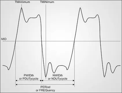
Figure 1: Horizontal-Axis Measurements
When acquiring Period and Frequency measurements their accuracy can be very much affected by the sample rate. Both of these measurements are calculated by counting the number of samples that occur between Middle crossings. If a 10 MHz signal is being sampled at 100 MHz, this will result in exactly ten samples per period. The samples at the zero crossings may be very near the borders. If one is missed, this results in only nine samples being detected which returns a Period of 9 * (10nsec) = 90 nsec and a resulting Frequency of 11.1 MHz. This resolution is obviously not very good. It could be improved by acquiring long waveforms to capture many cycles and average out the resolution error. Another solution would be to sample the signal at 1 GHz or greater. Overall, for more accurate Frequency and Period measurements, it is best to sample at a far greater rate than the signal and capture many cycles. Cycle Average and Cycle Frequency measurements can be used to measure only the first cycle if desired. Also, the gated methods described in the vertical-axis section can also be employed. All of these methods are still susceptible to the resolution errors described above.
Phase measurements make most sense when acquiring two or more waveforms to determine how many radians or degrees a waveform is shifted in relation to another. However, the phase can be measured on a single periodic signal. This can be confusing, but it is simply calculated by comparing the starting point of the waveform to the rising edge Middle crossing. Figure 2 shows one signal with a positive 90 degree (1.57 rad) phase shift and another with a 270 degree (4.72 rad) phase shift.
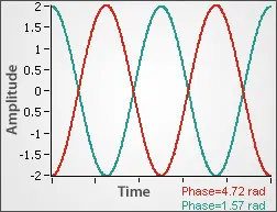
Figure 2: Phase Measurement
Edge Measurements
A subset of Horizontal-Axis measurements is Edge Measurements. All of these measurements are made in relation to the Reference High (REF HIGH), Reference Middle (REF MID), and Reference Low (REF LOW). These references are user-selectable and are different than the High, Middle, and Low levels discussed in the previous sections, which are not user-selectable. By default, the REF HIGH, REF MID, and REF LOW are set to 90%, 50%, and 10% of the Amplitude (High – Low). However, all of these percentages can be adjusted to suit the application’s needs, or input in terms of absolute voltages.
With a firm understanding of the references, the meaning of the edge measurements becomes clear. They are shown in Figure 3. The Rise Time (RTIMe) measures the relative time for the leading edge of a pulse to rise from the REF LOW to the REF HIGH. The Fall Time (FTIMe) measures the same thing on the falling edge. The Rise Crossing Time (RTCRoss) is the absolute time when the waveform rises above the REF MID, measured from the start of the waveform. The Fall Crossing Time (FTCRoss) measures the same thing on the falling edge. All four of these measurements are edge selectable, meaning that the user can choose which number edge to characterize within the capture window.
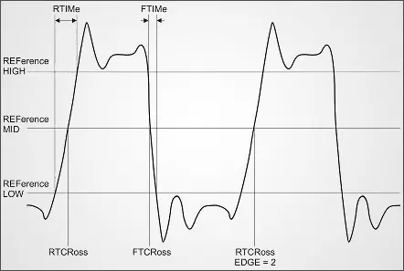
Figure 3: Edge Measurements
One possible problem when taking edge measurements are inaccurate crossings due to noise on the vertical axis. Figure 4 shows a signal with and without vertical noise and how that could affect a horizontal measurement. The noisy signal crosses the voltage thresholds at slightly different points than the smooth signal, causing a shorter Rise Time Measurement. Another problem with a noisy signal is the potential for false crossings. This occurs when noise causes a signal to dither near the crossing points in several recorded crossings. Both of these problems can be avoided by either oversampling and averaging or by using the Smooth function before taking the measurement to reduce the noise. The algorithms used on ZTEC oscilloscopes incorporate hysteresis at the crossings which helps avoid detecting false crossings. This does result in a minimal detectable edge, however.
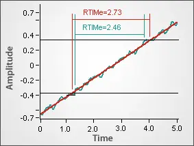
Figure 4: Noisy & Smooth Rise Times
Relative vs. Absolute Measurements
Much like the distinction made between absolute and relative voltage measurements made in the vertical-axis section, there are absolute and relative time measurements as well. For example, the Period of a waveform compares two points on the same waveform, so it’s often unnecessary to relate this to a real-world or absolute time. Therefore, this is considered a relative time measurement. An example where the absolute time would be important is measuring the Time of Maximum (TMAX), which returns the timestamp of the first maximum voltage level in relation to the start of the acquisition.
Source: ztecinstruments.com