Application Note 1553
Introduction
The quality of your oscilloscope’s display can make a big difference in your ability to troubleshoot your designs effectively. If your oscilloscope has a low-quality display, you may not be able to see critical signal anomalies. A scope that is capable of showing signal intensity gradations can reveal important waveform details, including signal anomalies, in a wide variety of both analog and digital signal applications.
This application note compares display quality for a variety of analog and digital signals using Agilent’s 6000 Series mixed signal oscilloscope (MSO) and LeCroy’s WaveSurfer 400 Series scope. In some examples, we also show the results displayed on a traditional analog oscilloscope. We also discuss a methodology for quantifying display quality to make it easier to compare scope displays objectively.
The third dimension: intensity modulation
Engineers traditionally think of digital storage oscilloscopes (DSOs) as two-dimensional instruments that graphically display only voltage versus time. But there is actually a third dimension to a scope: the z-axis. This third dimension shows continuous waveform intensity gradation as a function of the frequency of occurrence of signals at particular X-Y locations. In analog oscilloscope technology, intensity modulation is a natural phenomenon of the scope’s vector-type display, which is swept with an electron beam. Due to early limitations of digital display technology, this third dimension, intensity modulation, was missing when digital oscilloscopes began replacing their analog counterparts. Now, it is making a comeback.
Display intensity gradation can be extremely important when you are looking for signal anomalies, especially when you are viewing complex-modulated analog signals such as video, read-write disk head signals, and digitally controlled motor drive signals. Intensity gradation is also helpful in a wide variety of mixed-signal applications found in embedded microprocessor and microcontroller technologies common in the automotive, industrial, and consumer markets. But even when you are viewing purely digital waveforms, intensity gradation can show statistical information about edge jitter, vertical noise, and the relative occurrence of anomalies.
Recently, all major digital oscilloscope vendors have begun to provide z-axis intensity gradation – with varying degrees of success – in order to emulate the display quality of an analog oscilloscope.
Complex-modulated analog signal applications
If you are working with complex-modulated signals, you need a scope with sufficient display quality to let you look at the big picture and then zoom in to see the details.
Composite video signals
Many engineers are familiar with standard NTSC or PAL composite video signals, which are complex-modulated analog signals. Figure 1 shows one frame of composite video photographically captured from an analog oscilloscope's display. Even though the display “flickers” when you view this waveform at 5 ms/div, there is important information embedded within the displayed waveform envelope. An experienced video design engineer can quickly determine the quality of analog signal generation from this display.
Figure 2 shows an older digital oscilloscope display without z-axis intensity modulation. Although this scope has sufficient sample rate and memory depth to capture details of this signal even at 5 ms/div, all captured points are displayed with the same display intensity. Waveform detail within the signal’s envelope is visually lost. Given a choice between analog oscilloscope technology and older digital display technology, it’s no surprise that today’s video labs are filled with analog oscilloscopes!
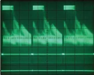
Figure 1. Full frame of composite video displayed on a 100-MHz analog oscilloscope
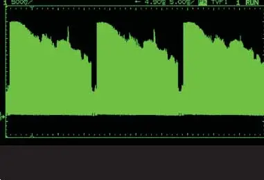
Figure 2. Full frame of composite video displayed on an older digital oscilloscope without intensity gradation capability
However, the visual quality of an analog oscilloscope’s display has finally been matched in a digital oscilloscope. Figure 3 shows the real-time capture of a video signal using Agilent’s 6000 Series oscilloscope. This scope uses Agilent’s proprietary MegaZoom III technology that provides up to 256 levels of color intensity gradation for each pixel based on deep memory acquisitions (up to 8 MB) mapped to a high-resolution display (XGA). This digital oscilloscope can display a repetitive analog signal with quality similar to (or perhaps better than) an analog oscilloscope, and it can also capture, display, and store complex single-shot signals with the same visual resolution. This is where conventional analog oscilloscopes fall short of their digital counterparts. Analogscopes can only display repetitive waveforms. Figure 4 shows a zoomed-in/windowed display of a single line of the composite video captured from the same acquisition that is shown in Figure 3. But since analog oscilloscopes can’t digitally store waveforms, we are unable to show a similar zoomed-in single-shot display using an analog oscilloscope.
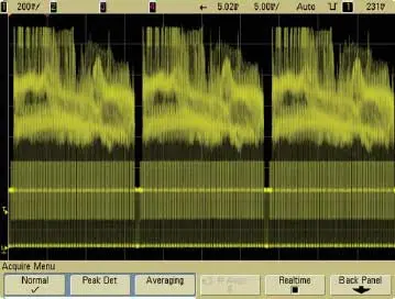
Figure 3. Full frame of composite video displayed on Agilent’s 60000 Series scope
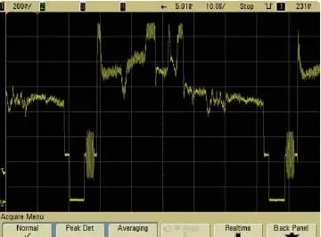
Figure 4. Zoomed-in display of a single line of video using Agilent’s 6000 Series scope
Figure 5 shows an attempt to repetitively capture this same composite video signal using a LeCroy WaveSurfer 400 Series oscilloscope. This oscilloscope has a special user-selectable display mode called Analog Persistence, which is a technique used by LeCroy in an attempt to emulate the display quality of an analog oscilloscope. With analog persistence, the intensity of digitized points decays over a user-specified persistence time. But with a minimum persistence setting of 0.5 seconds, the scope’s effective waveform update rate is just two waveforms per second. Although the quality of LeCroy’s analog persistence mode far exceeds that of older digital scopes (Figure 2), we think it falls short of the quality of either Agilent’s MegaZoom III technology or of an analog scope’s display quality. We encourage you to judge for yourself. But just like an analog oscilloscope, analog persistence in the LeCroy WaveSurfer 400 Series oscilloscopes is primarily a repetitive mode of operation. And although analog persistence does provide minimal levels of intensity grading for real-time acquisition displays, this display mode does not provide a display of continuous waveforms, but only displays “dots” as shown in Figure 6.
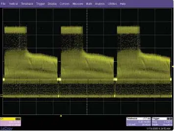
Figure 5. Full frame of composite video using the LeCroy WaveSurfer scope
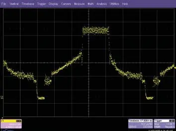
Figure 6. Zoomed-in display of a single line of video using the LeCroy WaveSurfer scope
Digitally controlled motor drive signal Another example of a complex analog signal is a digitally controlled motor drive signal. A one-time start-up cycle of a motor would be classified as a single-shot phenomenon. Figure 7 shows how Agilent’s 6000 Series mixed signal oscilloscope (MSO) is able to reliably capture one phase of this single-shot start-up motor drive signal. You can also use this scope’s digital/logic channels to synchronize and trigger the waveform capture based on the digital control signals of the motor. This capability can be extremely important when you attempt to synchronize acquisitions on not only power-up sequences, but also on particular motor positioning commands. Although not shown, this oscilloscope could just as easily capture all three phases of the motor drive signals simultaneously using its four channels of analog acquisition.
Also shown in Figure 7 are two zoomed-in images taken from the same single-shot acquisition. With this scope’s MegaZoom III technology, we can see a bright vertical vector (near the center of the display) in the middle image after zooming-in by a factor of 100. Further waveform expansion (20,000:1) on the pulse-width modulated (PWM) burst reveals a glitch, as shown in the image on the right.
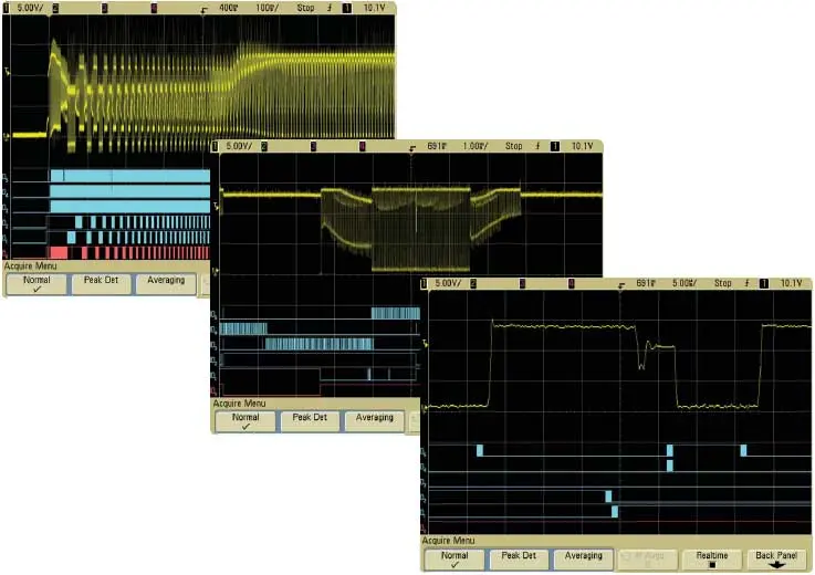
Figure 7. Motor drive signal start-up sequence with digital control signal triggering and various levels of zoom to reveal “runt” pulse using Agilent’s 6000 Series MSO
As shown in Figure 8, the LeCroy WaveSurfer oscilloscope is able to capture the start-up cycle of motor drive signal with some levels of intensity grading. However, when zooming in to observe waveform details, this oscilloscope lacks sufficient acquisition and display resolution to clearly show the signal anomaly that the Agilent oscilloscope captured and displayed. When zoomed in by a factor of 20,000 on this single-shot waveform capture, Figure 9 shows significantly less signal detail as compared to the Agilent 6000 Series oscilloscope. With just 2 M points of acquisition memory, the LeCroy scope captures this waveform with one-fourth the sample rate of the Agilent scope, which provides up to 8 M points of acquisition memory.
No attempt was made to capture this signal on an analog scope since our signal was single-shot and a conventional analog oscilloscope is incapable of storing a single-shot waveform. At this time base setting (100 ms/div), you would observe nothing more than a streak of light traveling across the analog scope’s display. And of course zooming in a stored waveform would be impossible with analog oscilloscope technology.

Figure 8. Start-up motor drive signal capture using a LeCroy WaveSurfer scope

Figure 9. Zooming in by a factor of 20,000 on the LeCroy WaveSurfer scope (note: dots have been enhanced for clarity)
Digital signal applications
The visual effects of a digital oscilloscope’s intensity gradation capability are most dramatic when you view complex-modulated analog signals such as the composite video and motor drive signals just shown. However, intensity gradation is also extremely important for uncovering signal anomalies when you are debugging digital circuitry. Figure 10 shows an example of uncovering a runt pulse embedded within a pulse-width modulated signal (PWM). The bright spot near the center of each burst is an indication that our scope has captured a signal anomaly. By zooming-in on one of the bright spots, we can clearly see details of the signal anomaly, as shown in Figure 11. Although an analog oscilloscope will also show the bright spots with repetitive sweeps, the analog scope is incapable of zooming-in on stored waveforms.
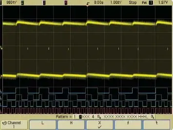
Figure 10. Agilent 6000 Series scope reveals “bright spots” buried within each digital burst
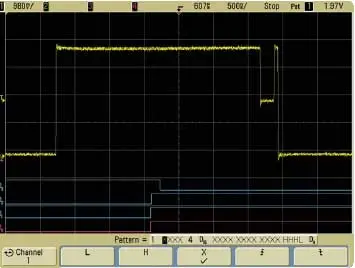
Figure 11. Zooming-in on a “bright spot” reveals a runt pulse
Figure 12 shows the LeCroy WaveSurfer’s attempt at capturing the same digital waveform information. This scope does not have sufficient display resolution to clearly show the bright spots, but merely shows a scattering of dots. However, with its 2 M points of acquisition memory, it does have sufficient acquisition resolution to show the runt pulse after zooming in on the waveform as shown in Figure 13. But without revealing the signal problem when observing waveforms on the longer time base range, you may never know that you need to zoom-in to observe this signal-fidelity problem.
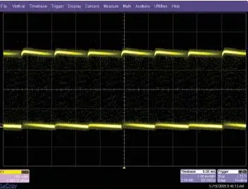
Figure 12. The LeCroy WaveSurfer scope fails to reveal embedded “bright spots”

Figure 13. Zooming-in on the waveform reveals the glitch
Display intensity gradation is also very important when you view waveforms that contain jitter, noise, and infrequent events. Levels of display intensity can help you interpret the relative frequency of occurrence of signal anomalies, and sometimes it can help you visually determine the type of jitter or noise in your system – based on display intensity dispersion – without resorting to sophisticated waveform analysis software.
Figure 14 shows an example of a digital signal that includes timing jitter (near the left side of screen), vertical noise (top and bottom of waveform), and a very infrequent glitch (near the center of screen). Because of the relative dimness of the displayed glitch, we know that this particular glitch occurs very infrequently. We can also see that the nature of the jitter is very complex and probably includes a large component of deterministic jitter (DJ). If the dispersion of display intensity on the signal’s edge appeared to be Gaussian in distribution, we would suspect that the jitter might be dominated by random jitter (RJ). For a more in-depth discussion on the different types of jitter, refer to Application Note 1448-2, “Finding Sources of Jitter with Real-Time Jitter Analysis,” listed at the end of this document.
Figure 15 shows the same signal displayed on an analog oscilloscope. Unfortunately, we are unable to show the jittering edge because it occurs before the trigger reference point (rising edge). But the signal edge that sometimes produces the infrequent glitch can be viewed. However, we can’t see the glitch on the analog scope’s display because it occurs too infrequently for conventional analog scope technology to display, even with the display intensity adjusted to full brightness.
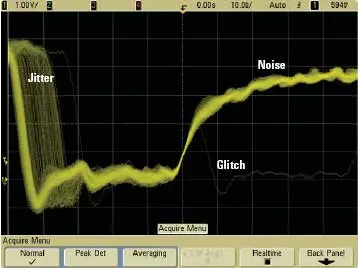
Figure 14. Display intensity gradation shows characteristics of jitter, noise, and signal anomalies on Agilent’s 6000 Series oscilloscope
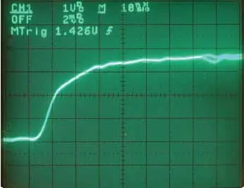
Figure 15. The analog oscilloscope fails to show the infrequent glitch
As shown in Figure 16, not only was the LeCroy WaveSurfer scope unable to clearly show the complex distribution of the jitter on the falling edge of this signal, but this scope was also unable to capture and display the infrequent glitch even though we held a probe on the test point for more than 30 seconds. However, the glitch capture problem was not due to insufficient display quality. The problem was associated with insufficient waveform update rates. For a more in-depth discussion on this important aspect of digital oscilloscopes, refer to Application Note 1551, “Improve Your Ability to Capture Elusive Events: Why Oscilloscope Waveform Update Rates are Important,” listed at the end of this document.
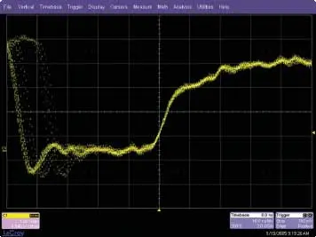
Figure 16. The LeCroy WaveSurfer scope fails to capture the infrequent glitch
Objectively evaluating oscilloscope display quality
The quality of an oscilloscope’s display is primarily a subjective issue. The best way to compare display quality between various digital oscilloscopes is to use them side-by-side and make visual comparisons using a variety of signals, as we have shown in this application note. Unfortunately, evaluating digital scopes from different vendors side-by-side is not always possible. Although there does not exist today a single oscilloscope specification that quantifies a scope’s display quality, there are three characteristics of an oscilloscope that contributes to quality-of-display that should be considered when evaluating the performance of an oscilloscope. These characteristics include: display resolution, number of intensity-graded levels for each pixel, and acquisition memory depth. All of these oscilloscope characteristics are specified in Agilent’s oscilloscope data sheets.
Display resolution is usually specified in the data sheet as the type of display such as an XGA display (768x1024) or a VGA display (640x480). Display resolution provides you with a relative indication of number of pixels utilized for waveform display. Although you might intuitively deduce that scopes with an XGA display have a display resolution of 786,000 pixels, not all pixels are actually used for waveform display. Some of the pixels are reserved for out-of-graticule menu graphics, plus with 8 bits of ADC vertical resolution, only 256 vertical pixels out of the possible 768 are used for real-time/non-averaged waveform display.
Besides maximum X-Y display resolution of the oscilloscope, another important factor is the number of intensity levels (z-axis) for each pixel. Without z-axis intensity modulation, complex waveforms will be displayed at a fixed display intensity, similar to the screen image shown in Figure 2 – regardless of the scope’s specified display X-Y resolution (XGA, VGA, etc). Agilent’s 6000 Series scopes are capable of displaying complex waveforms with 256 variable levels of intensity. Other scopes in this class only provide up to just 16 levels of pixel intensity grades.
The last factor to consider is acquisition memory depth. Although some scopes use repetitive sampling techniques to “fill-in” waveform complexity on the scope’s display using timed-persistence display modes, Agilent’s 6000 Series scopes with MegaZoom III technology are able to map up to 8,000,000 points to the display after each real-time acquisition. This amount of acquisition memory far exceeds the maximum number of pixels available for waveform display. This means that many of the pixels will receive multiple “hits” during each acquisition cycle. The number of hits then determines the level of intensity for each pixel. For example, if a particular pixel gets hit just one time, it receives the minimum viewable level of intensity. Pixels that receive 256 or more hits receive the maximum level of intensity. This means that with Agilent’s MegaZoom III technology, the 6000 Series oscilloscopes provide superior display quality for not only repetitive applications, but also single-shot/real-time measurement applications.
Summary
When considering the purchase of your next digital oscilloscope, don’t consider just bandwidth, sample rate, number of channels, and memory depth. Another very important criterion is display quality. An oscilloscope’s third dimension, the z-axis, which shows intensity gradation of signals based on frequency-of-occurrence, can reveal important waveform details, including signal anomalies, in a wide variety of both analog and digital signal applications. In this application note, we have attempted to show qualitative comparisons using Agilent’s MegaZoom III technology compared to both analog oscilloscope technology and LeCroy’s analog persistence display technology. In addition, we have discussed the three important characteristics of an oscilloscope that should be considered when evaluating a scope’s display quality.
To view an on-line video that demonstrates the importance of display quality and waveform update rates, go to www.agilent.com/find/scope-demo, and then click on the video titled, “Expanding Beyond Two Dimensions.”